How Ottawa–Gatineau was drawn
3,275 km² · 39,499 squares · 5 governments · 8 days · about CA$370 (US$263) spent
How it was made, in short
- One camera that never moves photographed Google’s 3D model of the region, one small square at a time. Three home computers drew all 39,499 squares, 3,275 km².
- A large image model repainted 300 squares in the style wanted. The 292 that passed every check were used to train a smaller painter, made for this project.
- That painter redrew every square on rented graphics cards. Automatic checks caught invented ponds and land painted over the river.
- Five governments share the open data (data anyone may reuse): the federal government (with the National Capital Commission), Ontario, Québec, the City of Ottawa and the Ville de Gatineau. Making both shores match took most of the work.
- Federal data tied it together. One laser survey, one height model, one weather service and the NCC’s paths cover both shores the same way.
- The work took eight days. It cost more than planned, and some things went wrong. All are listed below.
Read the full story
2 cities · 2 provinces · 5 governments · 2 languages · 2 transit agencies · 3,275 km² of map · 300 teacher paintings, 292 kept · 39,499 squares · 8 days · about 105 hours of rented graphics cards · about CA$370 (US$263) spent
Why it was made
The aim was a map of the whole capital region, drawn to look hand-made, with both shores at once. Earlier tiny-city maps such as isometric.nyc, tiny.london and Isometric Toronto each cover one city. A look at 119 of them in November found none that covered Ottawa and Gatineau together, or any two provinces. This one was built with Claude in 8 days.
Five governments, one map
Ottawa–Gatineau has five governments: the federal government (with the National Capital Commission, the NCC), Ontario, Québec, the City of Ottawa and the Ville de Gatineau. Each shares its data in its own way. Each has its own licence, which is the set of rules for reusing the data. A map that crosses the river has to join all five without showing the joins.
| Government | What it provided | How good it was | How the gaps were filled |
|---|---|---|---|
| Federal + NCC | A 1 m laser survey of the ground and a 30 m terrain model from Natural Resources Canada (NRCan), a national grid for converting heights, Environment Canada weather, NCC paths and remarkable trees | Strongest. It does not stop at the river, so both shores get the same quality. The NCC names things in both languages. | The yardstick for heights, water, weather and paths. |
| Ontario | DRAPE 2024 aerial photos (560 tiles of 1 km, sharp to 16 cm) and the 511 live road feed | Strong. Sharp photos. The photo order came with no licence file, so the licence rests on the order confirmation. | The photos help check water on the Ottawa side. The site’s server reads the feed, not the visitor’s browser. |
| Québec | Building outlines, the property assessment roll, official place and street names, a daily roadwork file, a heritage list | Good licences, partial data. Outlines have no heights. Laser scans are older and use an older height system. No aerial photos could be confirmed for use. | Heights come from the federal survey, the old height system is converted, and the roll gives building age in Gatineau. |
| City of Ottawa | Road lines, trees, street lights, traffic cameras and counts, addresses, heritage, public art, cycling | Richest. Detailed and current. No licence could be confirmed for its 3D building sets, so they are left out. | Ottawa’s real poles and roads are used to measure the Gatineau side. |
| Ville de Gatineau | Addresses and cycling paths | Thinnest. No tree list, street lights, city cameras, road closures or aerial photos. | Gaps are filled with OpenStreetMap, federal heights and estimates. The map says so. |
Sources and licences are in the Credits. Every source was logged before use: 70 entries, counting tools and fonts.
Ottawa’s side was the easiest to draw. Gatineau’s thinner data shaped the map most.
- Heights. Québec’s building file has outlines only. Its laser scans are older and use an older height system, CGVD28. So heights on both shores come from one federal survey, converted to the newer system (CGVD2013) with a national conversion grid (CGG2013). A tower in Hull and a tower in Ottawa are measured the same way. Québec’s property assessment roll adds building age for 86,770 Gatineau properties.
- Trees and street lights. Ottawa lists 240,334 trees and every light pole. Gatineau lists neither, and OpenStreetMap has only 431 lamps there. Gatineau’s poles are placed along its roads, at the spacing measured from Ottawa’s real poles. They are estimates, and the credits say so. Gatineau’s trees will come from a provincial map of wooded areas, which shows forests, not single trees.
- Roadwork, cameras and transit. Gatineau has no city cameras. Québec’s road-camera pictures have no reuse terms, so none are used. OC Transpo’s live feed shows buses only, so the O-Train runs from its timetable.
What tied the two shores together
Federal data does not stop at the river. Where a city or province covered one side, a federal source covered both, in the same form and quality.
- One flat river. NRCan’s HRDEM is a 1 m height model made from one laser survey of both cities. It gives each stretch of river one flat height: 41.3 m for the Ottawa River, 58.9 m for Lac Deschênes. That height decides what counts as water. Before, each square guessed its own water, and neighbours disagreed. With one shared rule, the pixels where neighbours disagreed fell from 9.16 million to 3.77 million, down 59%.
- The NCC, on both shores. Its paths and trails run through Gatineau Park and Québec’s urban lands as well as Ontario’s: 1,213 lines touch the map, 422 in Gatineau Park and 189 on Québec’s urban lands. Environment Canada’s weather covers both shores too.
Drawing every square
One map grid covers both shores. One camera was chosen and frozen. It looks north and is tilted 30 degrees down. Because it never moves, every square lines up with its neighbours to a fraction of a pixel. That lets thousands of separate paintings join into one map.
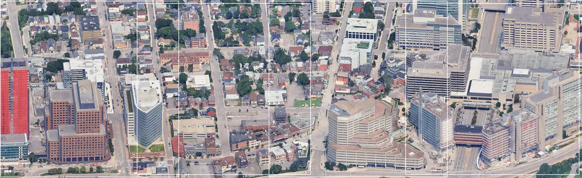
The final map has 39,499 squares and covers all of Ottawa and Gatineau, 3,275 km². Each square is drawn in headless Chromium, a web browser with no window. The 3D scenery is Google’s Photorealistic 3D Tiles, which arrive through Cesium ion.
The drawing ran on computers already at home, linked by Wi-Fi: two MacBooks (one with Apple silicon, 10 cores and 16 GB of memory; one with an Apple M4 chip and 16 GB) and an Asus laptop (AMD Ryzen 7 4800H, NVIDIA GTX 1650 graphics card, Windows 11). All three read one shared work list, kept in Cloudflare R2 online storage. A computer claims a square before drawing it, so none is drawn twice. A watchdog program pauses a computer when its memory runs low.
At its fastest, the three drew about 3,200 squares an hour. About 37,000 squares took 17 hours, from the morning of November 14 to the early hours of November 15, at no extra cost.
Teaching a painter
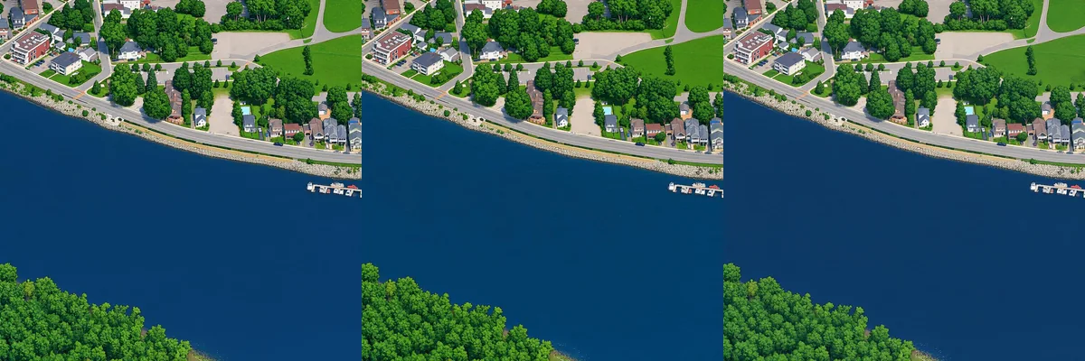
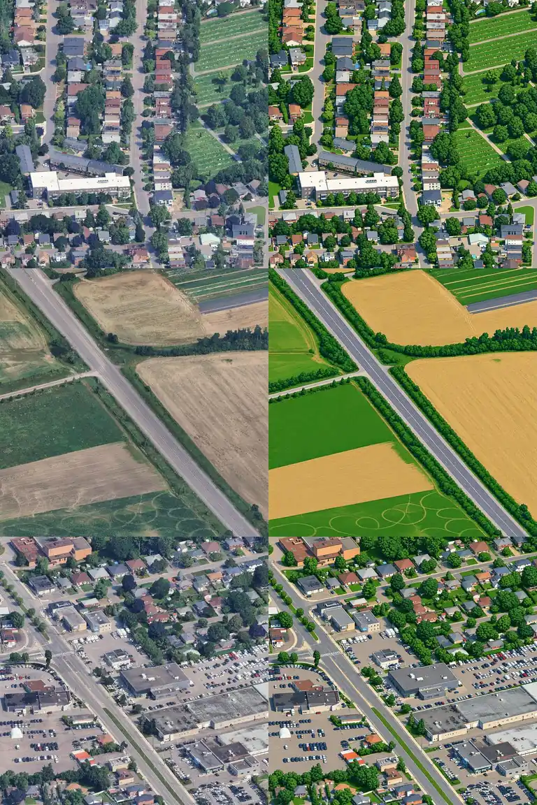
The goal was the crisp, calm look of a hand-drawn city map. A large commercial image model repainted 300 squares from across the region. Automatic checks looked for moved streets, changed water and invented details. 292 passed.
Painting the whole region with a commercial model would cost far too much. So the project trained its own painter: an open model, Qwen-Image Turbo, plus a small add-on that teaches it the style from the 292 pairs. Training took about 2 hours on one rented graphics card. Copies saved every 500 steps were compared side by side, and one was chosen.
Painting 39,499 squares
The first full run covered 14,257 squares. On one home computer, that would have taken one to two months. So up to 40 cloud machines for drawing and 10 graphics cards for painting were rented for a few hours. Each took the next square from a shared list.
It did not all go to plan. A bug made one batch run nearly three times longer than intended, and the first safety stop had a bug too. The bill came in higher than intended.
The final painting ran on up to 16 rented RunPod L40S graphics cards at once. The painter is Qwen-Image-2.1-Turbo with the project’s own style add-on. It works in 8 steps per square and cost about US$0.002 (CA$0.003) a square.
Checks and fixes
AI models like to add things, and this one sometimes painted ponds that do not exist. Every painting gets an automatic quality check. A second “verdict” check flags a town or detail invented over dark woods. Then an automatic water fix corrects the water, using real outlines from OpenStreetMap (a free map made by volunteers) and the federal ground model. On the Ottawa side, Ontario’s aerial photos add one more check. The water check found four invented ponds in the teacher’s paintings, and some of that habit carried into the painter.
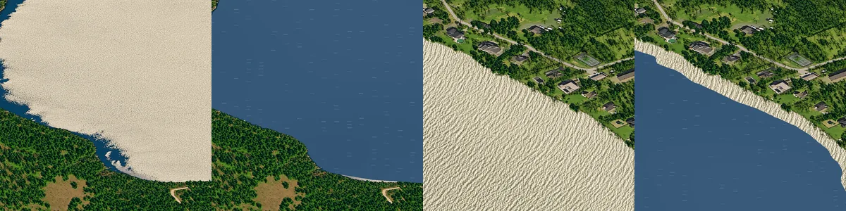
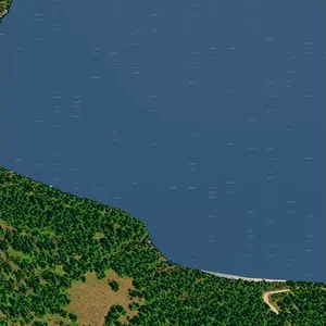
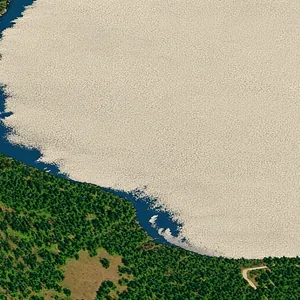
Google’s 3D model is broken in a few places. A square was flagged if its drawing sat more than 4 m off the federal ground model over water. Those squares were patched from good neighbours. 23 squares needed that. 10 Gatineau squares with small holes were filled the same way.
A browser loads only the part of the 39,499 pictures that is on screen. Computers get every place in a lossless image format (no quality lost). Phones get a lighter copy that loads faster. Both are served from Cloudflare’s network. The site is plain on purpose. It uses a Cloudflare Worker (a small program that runs online), R2 storage, a D1 database, OpenSeadragon (a viewer for zooming pictures) and Vite (a build tool).
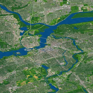 Downtown and both shores, about 7.5 km
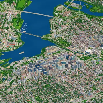 The city, about 1.9 km
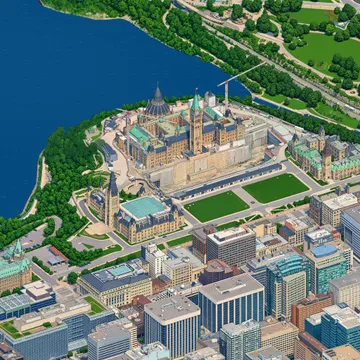 Parliament Hill, about 470 m
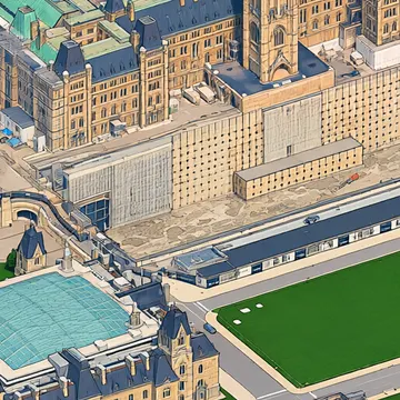 A building, about 120 m
Buses move because OC Transpo and the STO share their positions every few seconds. Rain and snow follow Environment Canada’s current weather, and night falls with the sun. One small server shares a single copy of it all, so the agencies see one visitor, not thousands.
What went wrong
- Every square once chose its own water, so neighbours disagreed. That left straight-line shores and wedges of land in the river. The shared water rule fixed most of it.
- A map formula drifted at the edges of the region. A setting mismatch spoiled the first test paintings. Both were fixed.
- Dark, leafless woods sometimes came out as an invented town. Some squares had land painted over the river. Brighter drawings and the real river outlines fixed them.
- The Gatineau side holds more guesses than the Ottawa side. Its street lights are estimated, and its heights come from a federal survey, not a city file. The map says so.
- The plan was CA$85. The total came to about CA$415 (US$293) all in, and about CA$370 (US$263) after Modal’s free credit, as the job grew from one city core to the whole region.
- The first cost guard read $0 every time because of a typing mistake in a script, and one drawing job ran past its planned stop.
What is still not right
Some mistakes remain. These crops come from the test run. The automatic checks flag many of them, but not all.
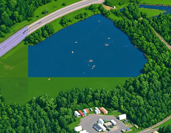
A seam. Two squares disagreed about a pond, so the join cuts it with a straight edge. The live map softens joins like this, but a faint blur can remain. 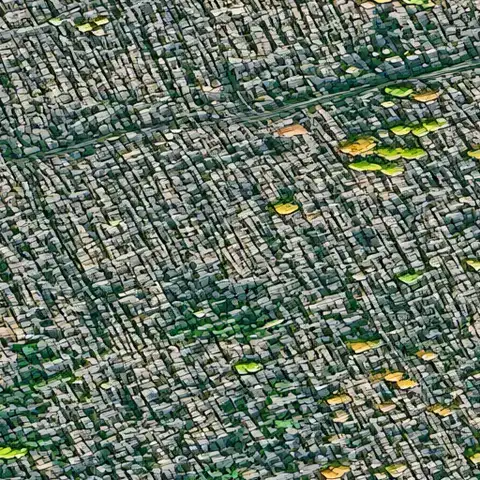
Bare woods. Trees without leaves in the 3D model come out grey and blocky. 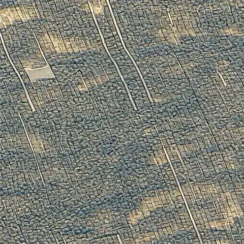
Tan ground. Bare fields and woods in the source imagery stay dull and patchy.
About 1 square in 100 failed the quality check twice, mostly rural forest that kept coming out as grey town. For now, those squares show as plain cream patches instead of a copy of the 3D drawing. A few squares at the very edge of Google’s data have holes and show as gaps. Zoomed far out, some straight lines show where areas painted on different days don’t quite match in colour.
Spotted one on the map? Use “Report a problem here”. Reports go straight to the maker.
What would change next time
- Test every cost guard on a tiny job before a big one.
- Rent cheaper graphics cards from the start. A check of other makers’ costs showed a much higher hourly price here, and the painter fits on a 48 GB card.
- Draw on cheaper machines from the start. The cloud drawing was far slower than other makers', and the home computers later did the same work for $0.
What it cost and how long it took
The money used came to about CA$370 (US$263), or less than 1 cent a square across all 39,499. Modal, the cloud service, also gave a free monthly credit of CA$42 (US$30), so the whole map is worth about CA$415 (US$293).
| Stage | Cost, CA$ (US$) |
|---|---|
| Teacher. Example paintings and style tests (OpenAI GPT Image, Google Gemini) | $52.84 (US$37.42) |
| Student. Training the project’s own painter, and test paintings to choose it | $16.56 (US$11.73) |
| Drawing, downtown. The Ottawa core, from Google’s 3D map (cloud computers) | $71.40 (US$50.56) |
| Painting, downtown. The Ottawa core (rented graphics cards) | $95.06 (US$67.31) |
| Painting, the rest. Gatineau, the suburbs and the countryside, and putting the map together (rented graphics cards and computers) | about $165 (US$116) |
| Drawing, the rest. About 37,000 squares on three home computers | $0 |
| Website. Domain for a year, and hosting so far | $15.09 (US$10.69) |
| All in | about $415 (US$293) |
| Modal’s free monthly credit | −$42 (−US$30) |
| Total used, after the credit | about $370 (US$263) |
Totals are as of November 16, 2026, rounded to the nearest CA$5. It keeps costing about CA$4 (US$3) a month to store the map, and about CA$15 (US$10) a year for the domain. Not counted: the Claude Ultra subscription and the basic ChatGPT and Gemini plans, which already existed, and the electricity of three home computers. In Canadian dollars, at the Bank of Canada exchange rate of November 9, 2026. The card was charged about 5% more on some payments because of conversion fees.
Eight calendar days, from the first line of code on November 8 to the finished map on November 15, 2026.
| When | What |
|---|---|
| Nov 8 | First drawing from Google’s 3D map. Camera fixed. Test area drawn: 458 pictures. |
| Nov 9 | Teacher paintings (292 good ones). Training of the painter in the evening. |
| Nov 10 | Whole Ottawa core drawn and painted overnight. Website up behind a password. Domain bought. |
| Nov 11 to 13 | Gatineau drawn and painted. Water, seams and layers fixed. |
| Nov 14 to 15 | The rest of the map: about 37,000 squares drawn in 17 hours on three home computers, then painted on rented graphics cards. |
| Nov 16 | Colours evened out between painted areas. About half of the blank patches repainted. |
| Machine time | about 105 hours of rented graphics cards, about 700 hours of cloud processors, about 17 hours on three home computers |
Machine time only, not working hours.
If you want to make one for your city
Start small: one neighbourhood, one frozen camera, a few hundred good teacher paintings. Spend the effort on checks, not on more paintings. And read the projects below first.
What’s next
- Seasons. Snow on the ground in winter, autumn colours, spring green.
- More angles. The whole city seen from four to six directions, so it can be turned around.
- Sharper up close. Newer painting models for more real detail, and a fix for the last squares: spring woods painted tan and a few invented ponds.
- Better Gatineau data. The Ville de Gatineau holds a list of about 17,000 trees, plus street lights, rink status, cameras and street closures. A request for open data could unlock them.
- A livelier city. Windows that light up at night, plus live river level, air quality, wildfire smoke and northern lights.
- More places and tours. Every place page with its own story, a winter tour, an O-Train tour, and old aerial photos to compare with today on the Ottawa side.
Earlier tiny-city maps
Tiny Capitale follows isometric.nyc by Andy Coenen, Isometric Toronto by John Fewell, tiny.london by Boris Starkov, Pixel Berlin and Pixel Singapore. The painting method owes most to Marcelo Eduardo’s open write-up on training small models to paint city tiles from 3D scenes. See Other tiny cities for the full list, and Credits for every source and licence.